1.7 Color spaces, and CIELAB in particular

To talk about mixing precisely we need coordinates for color. The ones used throughout these notes are CIELAB. Lightness (\({L^{*}}\)) runs from 0 for black to 100 for white. Two color coordinates run across it, one from green to red (\({a^{*}}\), negative for green and positive for red) and one from blue to yellow (\({b^{*}}\), negative for blue and positive for yellow), and a gray sits at zero on both. A color’s distance from the gray axis is its chroma (\({C^{*}_{ab}}\)), how vivid it is, and its angle around the axis is its hue angle (\({h_{ab}}\)), measured in degrees from the red direction. The coordinates come from the CIE’s three standard numbers by a fixed formula built on the opponent channels: the green-red coordinate is the red-green signal and the blue-yellow coordinate the yellow-blue one.

Looking straight down the lightness axis, as in Figure 6(a), shows where all 78 Golden paints in these notes fall on the plane of the two color coordinates when they are used straight from the tube. The yellows sit at the top, the reds to the right, the blues at the bottom and the greens to the left, and the farther a paint lies from the center, the more vivid its color. The dark transparent paints, the phthalos, the quinacridones and dioxazine, cluster near the center. Straight from the tube they are nearly black, and a near black has little chroma whatever its hue; their color appears only when they are thinned or mixed with white, as Section 3.4 explains.

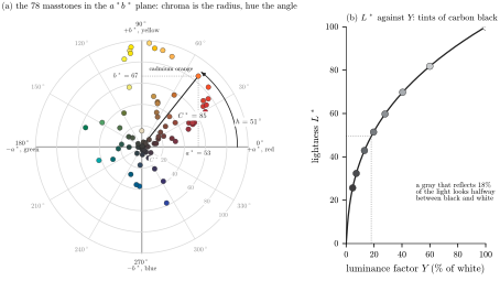
Figure 6. CIELAB. (a) The 78 Golden masstones in daylight, seen from above on the \({a^{*}}{b^{*}}\) plane, each drawn in its own color; for one paint, cadmium orange, the chroma (the distance from the center) and the hue angle are drawn in. (b) Lightness against the share of the light a surface reflects, with tints of carbon black in titanium white marked on the curve; the tints are computed with the mixing model.

Lightness does not grow in step with the amount of light. Panel (b) shows the relation: a gray that reflects only 18 percent of the light already looks halfway between black and white, and the remaining 82 percent of the light covers the other half of the lightness scale. This compression of value is necessary to accurately represent our visual perception. It means a small change in the light reflected is a bigger step of value among the darks than among the lights. The painter’s rule that a little black goes a long way in a tint comes mainly from the paint itself: near white, the first trace of an absorbing pigment takes away a large share of the light (Section 2.1).

Because CIELAB is built so that equal distances look roughly equally different, the difference between two colors can be measured as the distance between them, and a difference of about one unit is close to the smallest a careful observer can see [3]. The space is not perfectly even: the same distance looks larger among grays than among vivid colors. So these notes use a refined measure of difference called CIEDE2000, which weights the parts of a difference to match what people see [45, 67]. Its unit is what these notes call a unit of color difference, written \(\Delta E_{00}\) in the figures. More even spaces exist, but for paint mixing CIELAB is good enough, and every pigment manufacturer, Golden included, publishes in it. A CIELAB color is always measured against a white under a particular light, and in these notes the light is daylight unless stated otherwise.

One more way of drawing color comes up later: the CIE’s chromaticity diagram. It is a flat map of colors with the amount of light taken out, so a color and a darker or lighter version of it land on the same spot. The single wavelengths of the spectrum lie around its curved, horseshoe-shaped edge, violet at one end and red at the other, and white sits near the middle; where a color lies between white and the edge shows its hue and how pure it is. Its most useful property is that a mixture of two lights always lies on the straight line between them, so three lights can make exactly the colors inside the triangle they mark out. Mixtures of paints do not follow straight lines, on this map or any other, as Part 3 shows. The formulas for CIELAB, for color differences and for the chromaticity diagram are in the math box at the end of this lesson.

TipThe math behind this lesson

CIELAB, color differences and chromaticity. CIELAB was adopted by the CIE in 1976 [11, 62]. From the tristimulus values of a color, \(X\), \(Y\), \(Z\), and those of the reference white, \(X_n\), \(Y_n\), \(Z_n\), define

\[ {L^{*}} = 116\, f\!\left(\tfrac{Y}{Y_n}\right) - 16, \qquad {a^{*}} = 500\left[ f\!\left(\tfrac{X}{X_n}\right) - f\!\left(\tfrac{Y}{Y_n}\right)\right], \qquad {b^{*}} = 200\left[ f\!\left(\tfrac{Y}{Y_n}\right) - f\!\left(\tfrac{Z}{Z_n}\right)\right], \tag{5} \]

where \(f(t) = t^{1/3}\) for \(t > (6/29)^3\) and a straight line of matching slope below that, so that the formula behaves well near black. The cube root is the compression of Figure 6(b): a gray with \(Y = 0.18\) has \({L^{*}} = 49.5\). It descends from the Munsell value scale, which was fitted to judgments of equal lightness steps [58], and it is a fair approximation to the eye’s response over the range of ordinary surfaces. The chroma and hue angle are the polar coordinates of \(({a^{*}}, {b^{*}})\),

\[ {C^{*}_{ab}} = \sqrt{{a^{*}}^2 + {b^{*}}^2}, \qquad {h_{ab}} = \arctan\!\left({b^{*}} / {a^{*}}\right), \tag{6} \]

with the angle taken in the right quadrant so that it runs from \(0^{\circ}\) to \(360^{\circ}\). In Figure 6(a), cadmium yellow medium sits at \({b^{*}} = 98\) with a chroma of 98, pyrrole red at a chroma of 68, and cobalt blue at \({b^{*}} = -53\). The hue angles of the paints used most in Part 3 are hansa yellow medium \(83^{\circ}\), diarylide yellow \(72^{\circ}\), pyrrole red \(29^{\circ}\), quinacridone magenta \(9^{\circ}\), ultramarine blue \(302^{\circ}\), cobalt blue \(294^{\circ}\), phthalo blue (green shade) \(300^{\circ}\), phthalo green (blue shade) \(233^{\circ}\), permanent green light \(161^{\circ}\) and chromium oxide green \(139^{\circ}\).

The \({a^{*}}\) axis compares \(X\) with \(Y\) and the \({b^{*}}\) axis compares \(Y\) with \(Z\); since \(\bar{x}\) is a red-heavy combination of the cones and \(\bar{z}\) is almost the S-cone sensitivity, these are the opponent channels of Figure 3 in all but detail. The space is defined relative to a white, so the same surface has different coordinates under different illuminants. These notes use daylight D65 and the 1931 \(2^{\circ}\) observer unless stated otherwise, which puts its values within a few units of Golden’s own, published for the \(10^{\circ}\) observer [25].

The simplest measure of color difference, \(\Delta E_{ab}^{*}\), is the Euclidean distance \(\sqrt{\Delta{L^{*}}^2 + \Delta{a^{*}}^2 + \Delta{b^{*}}^2}\), and a difference of about 1 is near the threshold of visibility under good conditions [3]. The space is not quite uniform: equal distances look larger in the neutrals than in saturated colors and larger in some hues than others, as MacAdam’s ellipses had already shown in the chromaticity diagram [46]. The CIEDE2000 formula, whose differences are written \(\Delta E_{00}\) and are the units of color difference of the main text, corrects for this with weighting functions for lightness, chroma and hue and a term for the blue region [45, 67]; for small differences it is roughly comparable to \(\Delta E_{ab}^{*}\) in the neutrals and smaller than it in saturated colors. Spaces with better uniformity include CAM16-UCS [44] and OKLab [60], and no Euclidean space can be exactly right, since perceived differences do not add along a path the way distances do [7].

The chromaticity of a color is its \(XYZ\) with the brightness divided out, \(x = X/(X+Y+Z)\) and \(y = Y/(X+Y+Z)\). By Grassmann’s laws, mixtures of lights lie on straight lines in the \((x, y)\) plane. The single wavelengths trace its curved edge, and the straight line joining the two ends of that edge holds the purples.

Sources

[3] R. S. Berns, Billmeyer and Saltzman’s Principles of Color Technology, 4th ed., Wiley, 2019.

[7] R. Bujack, E. Teti, J. Miller, E. Caffrey and T. L. Turton, The non-Riemannian nature of perceptual color space, Proceedings of the National Academy of Sciences 119 (2022), e2119753119.

[11] CIE, Colorimetry, 4th ed., CIE 015:2018, Commission Internationale de l’Éclairage, Vienna, 2018.

[25] Golden Artist Colors, Inc., Heavy Body Acrylics: Pigment Detail Chart, https://goldenartistcolors.com, 2025.

[44] C. Li, Z. Li, Z. Wang, Y. Xu, M. R. Luo, G. Cui, M. Melgosa, M. H. Brill and M. Pointer, Comprehensive color solutions: CAM16, CAT16, and CAM16-UCS, Color Research and Application 42 (2017), 703–718.

[45] M. R. Luo, G. Cui and B. Rigg, The development of the CIE 2000 colour-difference formula: CIEDE2000, Color Research and Application 26 (2001), 340–350.

[46] D. L. MacAdam, Visual sensitivities to color differences in daylight, Journal of the Optical Society of America 32 (1942), 247–274.

[58] S. M. Newhall, D. Nickerson and D. B. Judd, Final report of the O.S.A. subcommittee on the spacing of the Munsell colors, Journal of the Optical Society of America 33 (1943), 385–418.

[60] B. Ottosson, A perceptual color space for image processing, https://bottosson.github.io/posts/oklab/, 2020.

[62] A. R. Robertson, The CIE 1976 color-difference formulae, Color Research and Application 2 (1977), 7–11.

[67] G. Sharma, W. Wu and E. N. Dalal, The CIEDE2000 color-difference formula: implementation notes, supplementary test data, and mathematical observations, Color Research and Application 30 (2005), 21–30.